Tidal Environments#
In chapter 4 of the textbook, we looked into the global variation in the main processes that shape the coast: wind, waves, and tides. In this notebook, we will focus on the large-scale variation in tides. The two main variables on the basis of which tidal environments can be classified are:
Magnitude of the tide, characterised by the tidal range;
Tidal character, determined by the importance of diurnal vs. semi-diurnal components
In this notebook, we will explore both classifications using python code. Therefore, please import the libraries that we need for the analysis from the cell below.
import pathlib
from pathlib import Path
import sys
from warnings import filterwarnings
import ipywidgets as widgets
from ipywidgets import interact
from matplotlib.patches import Patch
import matplotlib.pyplot as plt
import numpy as np
import pandas as pd
import cartopy.crs as ccrs
import xarray as xr
from datetime import datetime, timedelta
from IPython.display import display, Image
import math
import pandas as pd
import pooch
import pickle

F_data_fp = pooch.retrieve(
    "https://coclico.blob.core.windows.net/coastal-dynamics/02-tide/02_F_data.pkl",
    known_hash="eae7be0e7b44ed5b211e931bd6e5948e0aa8db067403956fe2d486f69e49c769",
)
F_data = pd.read_pickle(F_data_fp)

cwd = pathlib.Path().resolve()
proj_dir = cwd.parent.parent.parent  # this is the root of the CoastalCodeBook
sys.path.append(str(proj_dir))

from initialize.Tide_Initialize import questions_3a1, questions_3a2, plot_4timeseries_with_interactive_controls
Downloading data from 'https://coclico.blob.core.windows.net/coastal-dynamics/02-tide/02_F_data.pkl' to file '/home/runner/.cache/pooch/918dec1d06d7bc0691082dd30d324d60-02_F_data.pkl'.
---------------------------------------------------------------------------
KeyboardInterrupt                         Traceback (most recent call last)
Cell In[1], line 20
     17 import pooch
     18 import pickle
---> 20 F_data_fp = pooch.retrieve(
     21     "https://coclico.blob.core.windows.net/coastal-dynamics/02-tide/02_F_data.pkl",
     22     known_hash="eae7be0e7b44ed5b211e931bd6e5948e0aa8db067403956fe2d486f69e49c769",
     23 )
     24 F_data = pd.read_pickle(F_data_fp)
     26 cwd = pathlib.Path().resolve()

File ~/micromamba/envs/coastal/lib/python3.11/site-packages/pooch/core.py:239, in retrieve(url, known_hash, fname, path, processor, downloader, progressbar)
    236 if downloader is None:
    237     downloader = choose_downloader(url, progressbar=progressbar)
--> 239 stream_download(url, full_path, known_hash, downloader, pooch=None)
    241 if known_hash is None:
    242     get_logger().info(
    243         "SHA256 hash of downloaded file: %s\n"
    244         "Use this value as the 'known_hash' argument of 'pooch.retrieve'"
   (...)
    247         file_hash(str(full_path)),
    248     )

File ~/micromamba/envs/coastal/lib/python3.11/site-packages/pooch/core.py:807, in stream_download(url, fname, known_hash, downloader, pooch, retry_if_failed)
    803 try:
    804     # Stream the file to a temporary so that we can safely check its
    805     # hash before overwriting the original.
    806     with temporary_file(path=str(fname.parent)) as tmp:
--> 807         downloader(url, tmp, pooch)
    808         hash_matches(tmp, known_hash, strict=True, source=str(fname.name))
    809         shutil.move(tmp, str(fname))

File ~/micromamba/envs/coastal/lib/python3.11/site-packages/pooch/downloaders.py:240, in HTTPDownloader.__call__(self, url, output_file, pooch, check_only)
    238     progress = self.progressbar
    239     progress.total = total
--> 240 for chunk in content:
    241     if chunk:
    242         output_file.write(chunk)

File ~/micromamba/envs/coastal/lib/python3.11/site-packages/requests/models.py:820, in Response.iter_content.<locals>.generate()
    818 if hasattr(self.raw, "stream"):
    819     try:
--> 820         yield from self.raw.stream(chunk_size, decode_content=True)
    821     except ProtocolError as e:
    822         raise ChunkedEncodingError(e)

File ~/micromamba/envs/coastal/lib/python3.11/site-packages/urllib3/response.py:1060, in HTTPResponse.stream(self, amt, decode_content)
   1058 else:
   1059     while not is_fp_closed(self._fp) or len(self._decoded_buffer) > 0:
-> 1060         data = self.read(amt=amt, decode_content=decode_content)
   1062         if data:
   1063             yield data

File ~/micromamba/envs/coastal/lib/python3.11/site-packages/urllib3/response.py:949, in HTTPResponse.read(self, amt, decode_content, cache_content)
    946     if len(self._decoded_buffer) >= amt:
    947         return self._decoded_buffer.get(amt)
--> 949 data = self._raw_read(amt)
    951 flush_decoder = amt is None or (amt != 0 and not data)
    953 if not data and len(self._decoded_buffer) == 0:

File ~/micromamba/envs/coastal/lib/python3.11/site-packages/urllib3/response.py:873, in HTTPResponse._raw_read(self, amt, read1)
    870 fp_closed = getattr(self._fp, "closed", False)
    872 with self._error_catcher():
--> 873     data = self._fp_read(amt, read1=read1) if not fp_closed else b""
    874     if amt is not None and amt != 0 and not data:
    875         # Platform-specific: Buggy versions of Python.
    876         # Close the connection when no data is returned
   (...)
    881         # not properly close the connection in all cases. There is
    882         # no harm in redundantly calling close.
    883         self._fp.close()

File ~/micromamba/envs/coastal/lib/python3.11/site-packages/urllib3/response.py:856, in HTTPResponse._fp_read(self, amt, read1)
    853     return self._fp.read1(amt) if amt is not None else self._fp.read1()
    854 else:
    855     # StringIO doesn't like amt=None
--> 856     return self._fp.read(amt) if amt is not None else self._fp.read()

File ~/micromamba/envs/coastal/lib/python3.11/http/client.py:473, in HTTPResponse.read(self, amt)
    470 if self.length is not None and amt > self.length:
    471     # clip the read to the "end of response"
    472     amt = self.length
--> 473 s = self.fp.read(amt)
    474 if not s and amt:
    475     # Ideally, we would raise IncompleteRead if the content-length
    476     # wasn't satisfied, but it might break compatibility.
    477     self._close_conn()

File ~/micromamba/envs/coastal/lib/python3.11/socket.py:706, in SocketIO.readinto(self, b)
    704 while True:
    705     try:
--> 706         return self._sock.recv_into(b)
    707     except timeout:
    708         self._timeout_occurred = True

File ~/micromamba/envs/coastal/lib/python3.11/ssl.py:1314, in SSLSocket.recv_into(self, buffer, nbytes, flags)
   1310     if flags != 0:
   1311         raise ValueError(
   1312           "non-zero flags not allowed in calls to recv_into() on %s" %
   1313           self.__class__)
-> 1314     return self.read(nbytes, buffer)
   1315 else:
   1316     return super().recv_into(buffer, nbytes, flags)

File ~/micromamba/envs/coastal/lib/python3.11/ssl.py:1166, in SSLSocket.read(self, len, buffer)
   1164 try:
   1165     if buffer is not None:
-> 1166         return self._sslobj.read(len, buffer)
   1167     else:
   1168         return self._sslobj.read(len)

KeyboardInterrupt:
1. Tidal Environments#
The tidal wave is distorted by local differences in water depth and by the location and shape of land masses and large embayments. This results in a global variation in tidal range controlled by the large-scale coastal configuration. The tidal character expressed through mean spring tidal range:
Category |
Mean spring tidal range |
|---|---|
Micro-tidal |
< 2m |
Meso-tidal |
2m - 4m |
Macro-tidal |
> 4m |
The tidal character, on the other hand, is defined by the form factor F:
Category |
Value of F |
|---|---|
Semi-diurnal |
0 - 0.25 |
Mixed, mainly semi-diurnal |
0.25 - 1.5 |
Mixed, mainly diurnal |
1.5 - 3 |
Diurnal |
> 3 |
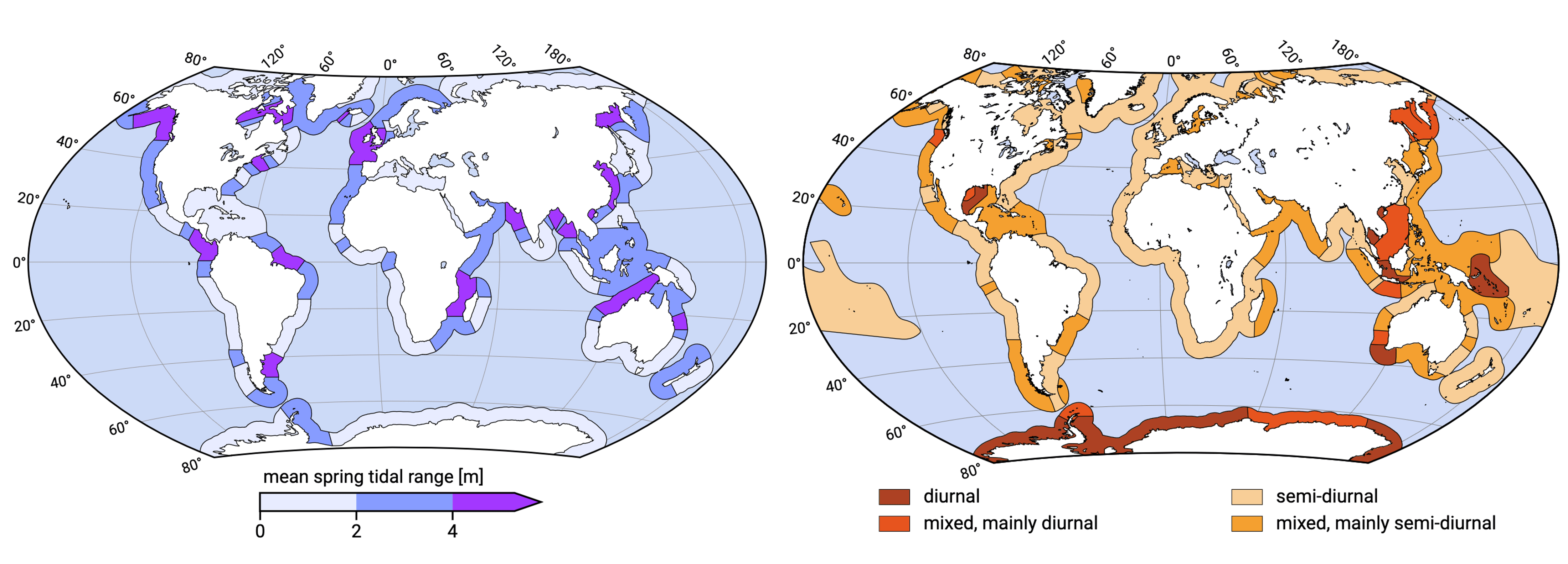
In the figure below, you can see the world distribution of mean spring tidal range (left) and tidal characters (right). The attribution of the tidal types follows J.L. Davies and Clayton (1980) (Figures 4.10 and 4.12 from the textbook).
Look into the semi-enclosed seas vs. open coasts; do you notice anything? Why?
Compare the two: do you notice any repetitive patterns? Hint: Look at the tidal range for specific tidal characters.

2. Tidal Character at Specific Locations#
Let’s now categorize the tide at four specific locations. We will once again use the FES2014 Global Tide data, which provides amplitude and phase information for 34 tidal constituents, distributed on 1/16˚ grids.
For each location, the amplitudes of the constituents that are needed to compute the form factor are shown in the table below.
Tidal amplitudes [cm] |
M2 |
S2 |
K1 |
O1 |
|---|---|---|---|---|
Scheveningen (Netherlands) |
75.78 |
17.74 |
8.39 |
11.85 |
Galveston (US Gulf of Mexico) |
13.08 |
3.97 |
16.17 |
15.89 |
Jakarta (Indonesia) |
4.58 |
5.18 |
25.75 |
13.46 |
Valparaiso (Chile) |
42.91 |
14.40 |
15.29 |
10.22 |
In cell below, write your own code to calculate the form factor F at each location.
# Write your code here.
# Run to get questions

print("\n What is the category of:")
questions_3a1()
Let’s now plot the tidal characters across the globe obtained from the FES2014 dataset and mark the four locations from above. Do your answers match the locations on the map?
## FES2014 Tidal Characters
# the code is a bit slow, it is doing a global contour!

# Define the categories and corresponding colors
categories = {
    'Diurnal': {'min': 3, 'max': float('inf'), 'color': '#ad4123'},
    'Mixed, mainly diurnal': {'min': 1.5, 'max': 2.9, 'color': '#e7541e'},
    'Mixed, mainly semidiurnal': {'min': 0.25, 'max': 1.49, 'color': '#f4a030'},
    'Semidiurnal': {'min': 0, 'max': 0.249, 'color': '#f8ce97'}
}

# Create a figure and axis
fig, ax = plt.subplots(figsize=(15, 13), subplot_kw={'projection': ccrs.Robinson(central_longitude=0.0)})
ax.set_global()

# Plot the scatter points with specific colors for each category
legend_patches = []
for category, values in categories.items():
    subset_data = F_data[(F_data['F'] >= values['min']) & (F_data['F'] <= values['max'])]
    if not subset_data.empty:
        scatter = ax.scatter(subset_data.index.get_level_values('lon').values,
                             subset_data.index.get_level_values('lat').values, s=1, color=values['color'],
                             label=category, transform=ccrs.PlateCarree())
        legend_patches.append(Patch(color=scatter.get_facecolor()[0], label=category))

# Add markers for specific locations - here you can edit the code if you are wondering for a specific location
locs = {
    'Scheveningen': [4.25, 52.125],  # lon, lat
    'Galveston': [-94.6875, 29.25],
    'Valparaiso': [-71.625, -33],
    'Jakarta': [106.8125, -6.0625],
}

for loc, coordinates in locs.items():
    lon, lat = coordinates
    ax.scatter(lon, lat, color='black', s=10, transform=ccrs.PlateCarree(), zorder=4)
    ax.text(lon - 25, lat+3, loc, color='black', fontsize=12, fontweight='bold', transform=ccrs.PlateCarree())

ax.legend(handles=legend_patches, loc='lower center', bbox_to_anchor=(0.5, -0.2), ncol=2, fontsize=12)
ax.coastlines(resolution='110m', color='black', linewidth=0.5)

plt.show()
Compare this figure to the tidal characters illustration mentioned earlier (Figure 4.12 in the textbook). What could be the reasons behind the observed differences?
3. Variation of Tidal Constituents#
Now that we’ve identified the tidal characteristics of each location, we can visualize their tidal constituents and address various questions.
Execute the block below to generate an interactive figure. The figure displays the individual tidal components (upper plot) and their combined tidal signal (second plot) for four locations, each characterized by distinct tidal behaviours.
You can adjust the plotted time range using the slider (from 1 day to 1 year) and select which tidal constituents to display with tick boxes. This allows you to experiment with different constituents, observe the resulting signals, and compare the locations.
# Choose tidal constituents
comps = ['M2', 'S2', 'N2', 'K2',  #semi-diurnal
         'K1', 'O1', 'P1', 'Q1',  #diurnal
         'MM', 'MF', 'SSA',       #long period
         'M4', 'M6', 'S4', 'MN4'] #short period (overtides)

# We choose one year to plot, 2000-2001 same as in the previous Notebook
dates = np.array([
    datetime(2000, 1, 1, 0, 0, 0) + timedelta(seconds=item * 3600)
    for item in range(24*365) #1 year
])

# download and load tidal signals
scheveningen_fp = pooch.retrieve(
    "https://coclico.blob.core.windows.net/coastal-dynamics/2_wind_waves_tides/tide_scheveningen.p",
    known_hash="4ebac210fc0893e52655cbc3c9501a6c805e3537f327fed7edb9e7dbfe7fa06a",
)
galveston_fp = pooch.retrieve(
    "https://coclico.blob.core.windows.net/coastal-dynamics/2_wind_waves_tides/tide_galveston.p",
    known_hash="26af20b240804a18a939d477632b4507d44ebdc98510deb07e601732c0846224",
)
jakarta_fp = pooch.retrieve(
    "https://coclico.blob.core.windows.net/coastal-dynamics/2_wind_waves_tides/tide_jakarta.p",
    known_hash="7950246c47e757d9dd427063d7c809fda4267ed119efd18de43237aa9f98c9c6",
)
valparaiso_fp = pooch.retrieve(
    "https://coclico.blob.core.windows.net/coastal-dynamics/2_wind_waves_tides/tide_valparaiso.p",
    known_hash="a19a51e3607822bc72ab902f83990d2b318a08d1982c25461f8ffd6e5caae35f",
)
with open(scheveningen_fp, 'rb') as pickle_file:
    scheveningen = pickle.load(pickle_file)
with open(galveston_fp, 'rb') as pickle_file:
    galveston = pickle.load(pickle_file)
with open(jakarta_fp, 'rb') as pickle_file:
    jakarta = pickle.load(pickle_file)
with open(valparaiso_fp, 'rb') as pickle_file:
    valparaiso = pickle.load(pickle_file)

tide = {
    'Scheveningen': scheveningen,
    'Valparaiso': valparaiso,
    'Jakarta': jakarta,
    'Galveston': galveston,
    }

plot_4timeseries_with_interactive_controls(comps, dates, tide)
# We start with the main constituents preselected
Set the time range to around 30 days and
a) select only the main semi-diurnal components
b) select only the main diurnal components
c) select only one semi-diurnal (M2) and one diurnal (K1) component
What kind of signal do you see for each location? Why are there differences between locations? Don’t forget to look at the y-axis range.
We also know that there are much longer variations than the ones above. Set the time range to the whole year and
a) select only S2 and K2
b) select only K1 and P1
What kind of combined signal can you see now?
Finally activate all components, including some short period constituents that we will further explore next week. Analyse the combined signals. What are the dominant components at each location?
4. Tidal Beating#
Using the knowledge gained from Chapter 3 of the textbook and the interactive figure above, try to answer the questions below. You can use the next cell as a calculator. Give your numeric answer with at least three significant figures.
Tidal constituents |
Name |
Equil. |
Period [h] |
|---|---|---|---|
Semi-diurnal |
|||
Principal lunar |
M2 |
0.24 |
12.4206012 |
Principal solar |
S2 |
0.11 |
12 |
Lunar elliptical |
N2 |
0.046 |
12.65834751 |
Lunar-solar declinational |
K2 |
0.031 |
11.96723606 |
Diurnal |
|||
Lunar-solar declinational |
K1 |
0.14 |
23.93447213 |
Principal lunar |
O1 |
0.10 |
25.81933871 |
Principal solar |
P1 |
0.047 |
24.06588766 |
Lunar elliptical |
Q1 |
0.019 |
26.868350 |
Long period |
|||
Fortnightly |
Mf |
0.042 |
327.8599387 |
Monthly |
Mm |
0.022 |
661.3111655 |
Semi-annual |
Ssa |
0.019 |
4383.076325 |
# Write your code here to get answers to questions 1 and 2. Use the values from the table above
# and use at least 3 significant figures.
# Run to get questions.
# The following answers are interchangeable, so do not put the same answer twice - this will result in a false correct answer.
# TC1, TC2
# TC3, TC4
# Month1, Month2
# TC5, TC6
# Month3, Month4
# TC7, TC8

questions_3a2()
