Wave dispersion and grouping#
%run initialize/init_2b.ipynb
Packages successfully loaded
Wind-generated and tidal waves can travel great distances until they finally reach the coast. In this section, we discuss the propagation of both individual waves and the behaviour of a group of waves together. It is recommended to read chapter 3 of the book Coastal Dynamics when studying this codebook.
1) Dispersion relation for tsunami waves#
The dispersion relation can be used for all kinds of waves, including tsunami waves. Can you assess the characteristics of tsunami waves at various water depth classifications? The questions are equivalent to the question in footnote 2 on page 114 of the textbook. You can use previously created functions and the cell below for answering.
W2_Q6()
# You can use this cell to answer the question

h = 4000
T1 = 5 * 60 # 5 min
T4 = 60 * 60 # 60 min

Q0 = 'Between which periods are tsunami waves at intermediate depth, according to the dispersion relationship?'
L_lower = h/0.5
k_lower = 2*np.pi/L_lower
w_lower = (9.81*k_lower*np.tanh(k_lower*h))**0.5 # dispersion relationship
T_lower = 2*np.pi/w_lower
L_up = h/0.05
k_up =2*np.pi/L_up
w_up = (9.81*k_up*np.tanh(k_up*h))**0.5
T_up = 2*np.pi/w_up
answer0 = round(T_up,1), round(T_lower,1)
print(Q0, '\n',answer0, 's', '\n')

Q1 = "What is the wavelength of the tsunami wave at those 4 points?"
L1 = wave_length(T=T1, h=h)
L2 = h / 0.5
L3 = h / 0.05
L4 = wave_length(T=T4, h=h)
Q1_answers = round(L1 / 1000, 1), L2 / 1000, L3 / 1000, round(L4 / 1000, 1)
print(Q1, '\n', Q1_answers, 'km', '\n')

Q2 = "What is the wave period of the tsunami wave at those 4 points?"
w1 = 2 * np.pi / T1
w2 = dispersion(k=2*np.pi/L2, h=h)
w3 = dispersion(k=2*np.pi/L3, h=h)
w4 = 2 * np.pi / T4
T2 = 2*np.pi/w2
T3 = 2*np.pi/w3
print(Q2, '\n',T1, round(T2,1), round(T3,1), T4 , 's', '\n')

Q3 = "What is the wave celerity (c) of the tsunami wave at those 4 points?"
c1 = L1 / T1
c2 = L2 / T2
c3 = L3 / T3
c4 = L4 / T4
print(Q3, '\n',round(c1,1), round(c2,1), round(c3,1), round(c4,1) , 'm/s', '\n')

Q4 = "What is the wave group velocity (cg) of the tsunami at those 4 points?"
k1 = 2 * np.pi / L1
k2 = 2 * np.pi / L2
k3 = 2 * np.pi / L3
k4 = 2 * np.pi / L4

n1 = 0.5 + k1 * h / np.sinh(2 * k1 * h)
n2 = 0.5 + k2 * h / np.sinh(2 * k2 * h)
n3 = 0.5 + k3 * h / np.sinh(2 * k3 * h)
n4 = 0.5 + k4 * h / np.sinh(2 * k4 * h)

cg1 = c1 * n1
cg2 = c2 * n2
cg3 = c3 * n3
cg4 = c4 * n4
Q4_answers = round(cg1, 1), round(cg2, 1), round(cg3, 1), round(cg4, 1)
print(Q4, '\n', Q4_answers, 'm/s')
Between which periods are tsunami waves at intermediate depth, according to the dispersion relationship?
 (410.4, 71.7) s

What is the wavelength of the tsunami wave at those 4 points?
 (57.6, 8.0, 80.0, 713.0) km

What is the wave period of the tsunami wave at those 4 points?
 300 71.7 410.4 3600 s

What is the wave celerity (c) of the tsunami wave at those 4 points?
 192.1 111.6 194.9 198.0 m/s

What is the wave group velocity (cg) of the tsunami at those 4 points?
 (180.9, 57.1, 188.8, 198.0) m/s
2) Dispersion relation in the cross-shore direction#
Both the water depth and the wave period influence the wave propagation speed, as we have seen in the previous question. In deep water, the depth is so large relative to the wavelength that the orbital velocities of the wave do not reach the bottom and no interaction between the waves and the bed is possible. In this case, the wave celerity is only affected by the wave period. The other extreme is in shallow water, where only the water depth influences the wave celerity, and the wave period is irrelevant (non-dispersive waves). Thus, two waves of different periods but at the same location have the same celerity if both waves meet the requirements for shallow water conditions. Only if the water depth for one or both of these waves is classified as intermediate or deep water, the waves have a different celerity.
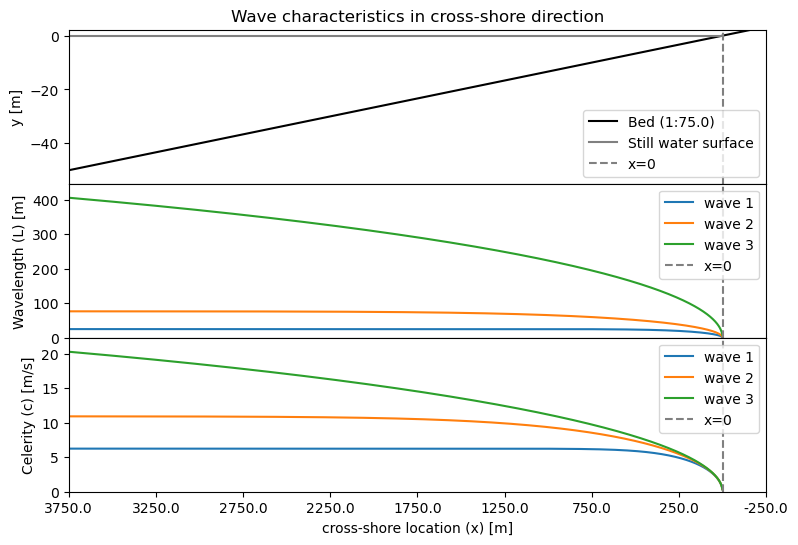
The wave celerity and the wavelength change when waves propagate in the cross-shore direction. In the interactive graph below you can study the impact of changing the bed slope (1:x) and the water depth (at the most seaward point) on the three waves (components). Here you will see that waves might have a different water depth classification (deep/intermediate/shallow) at the same time and location. Below the graph are a few practical questions that assess the effect of wave period, depth, and bathymetry on the wavelength and period.
W2_Q7()

# You can use this cell for computations

# No computations are needed, the line is straight in deep water and overlapping in shallow water.
answer1 = 'wave1' + 'wave2'
answer2 = 'wave2' + 'wave3'
answer3 = None
3) Wave groups#
Multiple waves (components) can coexist, influencing the sea surface elevation, currents, etc. The sea surface elevation can be described by substituting the harmonic components, as expressed in formula 1.
\begin{equation} \tag{1} \eta = a_1 sin(w_1t-k_1x) + a_2 sin(w_2t-k_2x) \end{equation}
This can be rewritten to formula 2, when \(a_1 = a_2 = a\).
\begin{equation} \tag{2} \eta = 2a sin(\frac{\omega_2+\omega_1}{2}t - \frac{k_2+k_1}{2}x)cos(\frac{\omega_2-\omega_1}{2}t-\frac{k_2-k_1}{2}x) \end{equation}
Which can be expressed in terms of differences (\(\Delta\)) and averaged values (indicated with a bar) for the radial frequency and wave number, resulting in:
\begin{equation} \tag{3} \eta = 2a sin(\bar\omega t - \bar k x)cos(\frac{\Delta\omega}{2}t - \frac{\Delta k}{2}x) \end{equation}
This formula consists of two parts, a slowly varying amplitude with \(2a cos(\frac{\Delta\omega}{2}t - \frac{\Delta k}{2}x)\) and a carrier wave through \(sin(\bar\omega t - \bar k x)\). Which contains the group length through \(\Delta k = 2 \pi/L_{group}\) and the group period from \(\Delta \omega = 2 \pi/T_{group}\).
3.1) Waves with same wave amplitude#
W2_Q9()
3.1.1) Time series of water elevation#
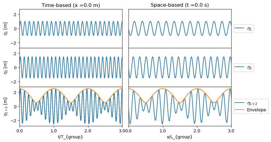
Below is the beginning of three functions, to calculate the water elevation at a single point in space, and the corresponding varying amplitude and wave envelope. The outcome of these functions will be plotted when you run the cell below. The top graph will check the outcome of eta_t(), and the bottom graph will show you all three functions on top of each other.
a1, a2, T1, T2 = 0,0,0,0
def eta_t():
    ...
    return eta

def varying_amplitude_t():
    ...
    return ...

def envelope_t():
    ...
    return ...

Show_Q9A()

# possible answer
print('Start output of the answer.')

# This is only for here, students have to define them manually
a1, a2, T1, T2, L1, L2, x_max, xp, t_max, tp, L_group, T_group = W2_Q9_param

def eta_t(a1,a2,T1,T2,L1,L2,t,xp):
    eta1_T = a1*np.sin(2*np.pi/T1*t-2*np.pi/L1*xp)
    eta2_T = a2*np.sin(2*np.pi/T2*t-2*np.pi/L2*xp)
    eta_T = eta1_T + eta2_T
    return eta_T

def varying_amplitude_t(a1,a2,T1,T2,L1, L2, t, xp):
    w1 = 2*np.pi/T1
    w2 = 2*np.pi/T2
    k1 = 2*np.pi/L1
    k2 = 2*np.pi/L2
    Delta_w = np.abs(w1-w2)
    Delta_k = k2 - k1
    var_amp = (a1 + a2)*np.cos(0.5*Delta_w*t - 0.5*Delta_k*xp)
    return var_amp

def envelope_t(a1,a2,T1,T2,t):
    envelope = np.abs( varying_amplitude_t(a1,a2,T1,T2,L1, L2, t, xp) )
    return envelope

Show_Q9A()
Almost there, your function varying_amplitude_t can not be plotted, please try to fix the bug.
Almost there, your function envelope_t can not be plotted, please try to fix the bug.
Almost there, your function eta_t can not be plotted, please try to fix the bug.
Start output of the answer.
3.1.2) Spatial distribution of the water elevation#
Use this code to make a plot to make a spatial distribution of the water elevation. The structure of this question is similarly as that one for the timeseries.
def eta_x():
    ...
    return eta

def varying_amplitude_x():
    ...
    return ...

def envelope_x():
    ...
    return ...

Show_Q9B()

# possible answer
print('Start output of the answer.')

# This is only for here, students have to define them
a1, a2, T1, T2, L1, L2, x_max, xp, t_max, tp, L_group, T_group = W2_Q9_param

def eta_x(a1,a2,T1,T2,L1,L2,tp,x):
    eta1_X = a1*np.sin(2*np.pi/T1*tp-2*np.pi/L1*x)
    eta2_X = a2*np.sin(2*np.pi/T2*tp-2*np.pi/L2*x)
    eta_X = eta1_X + eta2_X
    return eta_X

def varying_amplitude_x(a1,a2,T1,T2,L1, L2, tp, x):
    w1 = 2*np.pi/T1
    w2 = 2*np.pi/T2
    k1 = 2*np.pi/L1
    k2 = 2*np.pi/L2
    Delta_w = np.abs(w1-w2)
    Delta_k = k2 - k1
    var_amp = (a1 + a2)*np.cos(0.5*Delta_w*tp - 0.5*Delta_k*x)
    return var_amp

def envelope_x(a1,a2,T1,T2,L1, L2, tp, x):
    envelope = np.abs( varying_amplitude_x(a1,a2,T1,T2,L1, L2, tp, x) )
    return envelope

Show_Q9B()
Almost there, your function varying_amplitude_x can not be plotted, please try to fix the bug.
Almost there, your function envelope_x can not be plotted, please try to fix the bug.
Almost there, your function eta_x can not be plotted, please try to fix the bug.
Start output of the answer.
3.1.3) Theory question#
Q10()
3.2) Waves with diffent wave amplitude#
The variable amplitude shows a sinusoidal pattern when the wave amplitudes are equal. The amplitude does not go to zero when different wave amplitudes are used, since they don’t cancel each other out at the nodes. The Hilbert Transform can calculate the wave amplitude when \(a_1\) and \(a_2\) differ. This transformation goes beyond the content of this course but is applied in the interactive graph below which shows the temporal and spatial signal for two different wave components. Feel free to use this graph to analyse the wave signals for various conditions.
W2_wave_groups()

Q11()
W2_Q12()
T1 = 7    # Wave period 1 [s]
T2 = 6.2  # Wave period 1 [s]
h = 20    # water depth [m]

Delta_k = ...
Delta_w = ...

Check_W2_Q12A()

#### begin answer
print('\n Begin output of the answer')
T1 = 7    # Wave period 1 [s]
T2 = 6.2  # Wave period 1 [s]
h = 20    # water depth [m]

# The calculation
L1 = wave_length(T1, h
                )
L2 = wave_length(T2, h)
k1 = 2*np.pi/L1
k2 = 2*np.pi/L2
w1 = 2*np.pi/T1
w2 = 2*np.pi/T2

Delta_k = np.abs(k2-k1)
Delta_w = np.abs(w2-w1)

Check_W2_Q12A()
# The answers are given after 3 attempts, the counter resets when running W2_Q12()
Begin output of the answer
Can you also calculate the group velocity (c_group), the wave group length (L_group), and the wave group period (T_group)?
c_group = ...
L_group = ...
T_group = ...

Check_W2_Q12B()
#### begin answer
print('\n Begin output of the answer')

c_group = Delta_w/Delta_k
L_group = 2*np.pi/Delta_k
T_group = 2*np.pi/Delta_w

Check_W2_Q12B()
Begin output of the answer
Here are some follow-up questions,
How many waves are there (approximately) in the wave group in space and in time?
Can you set the graph above such that the number of waves in the group in space and time are equal?
When is the difference between the number of waves in a group for space and time about a factor of 2?
Below is a graph that shows two wave components propagating. You can define the amplitude and period of two wave components and set the water depth. (Not the wavelength) You can zoom in and out to obtain a specific number of waves of the wave group on the x-axis by setting “n_waves group”. The Hilbert Transform is applied to show the variable wave amplitude.
Can you find out when the waves are dispersive and when not? How is this visible on the graph?
Unfortunately is the graph very computationally demanding, resulting in low frames per second, so it is a challenge to see the action, but you might think of the correct reasoning.
W2_Wave_animation()
